Loading required package: pacmanSeeing the Unseen
Predicting Brain Stroke in a Patient
Abstract
Strokes are a significant public health concern worldwide, and predicting the risk factors associated with strokes can contribute to early intervention and improved patient outcomes. This project aims to implement classification models on a data pertaining to stroke occurrences and check which has the highest accuracy. We then want to use the best model to rank the significance of each feature.
Introduction
The emergence of advanced healthcare datasets has paved the way for groundbreaking research and development in the realm of medical science. In our pursuit of leveraging data-driven insights to address critical health issues, we have undertaken a comprehensive analysis of the Brain Stroke Dataset sourced from Kaggle. This dataset, offers a rich repository of patient records and associated attributes, presenting a unique opportunity for in-depth examination and exploration.
The primary impetus behind this project is the compelling need to revolutionize early stroke detection and refine risk assessment methodologies. Brain strokes, with their potentially devastating consequences, underscore the significance of timely intervention. By harnessing the power of data analytics, we aim to unravel patterns and correlations within the dataset that can contribute to the development of predictive models. These models, in turn, hold the potential to augment healthcare professionals’ ability to identify individuals at risk of strokes at an early stage.
Question 1: How accurate are various classification models for detecting a stroke in a patient?
Approach
In the initial phase of our brain stroke prediction project, we conducted comprehensive examination of the dataset. The brain.shape and brain.info() checks ensured the dataset’s integrity, revealing its dimensions and basic information. Notably, no missing values were found (brain.isnull().sum()).
Visualizations were created to delve into correlations, including work types and smoking statuses, and the likelihood of heart disease based on gender, age, and work type.
We develoepd classification models using Logistic Regression, K-Nearest Neighbors, Random Forest and Decision Tree and picked the best model in based on accuracy value.
Exploratory Analysis and Visualizations
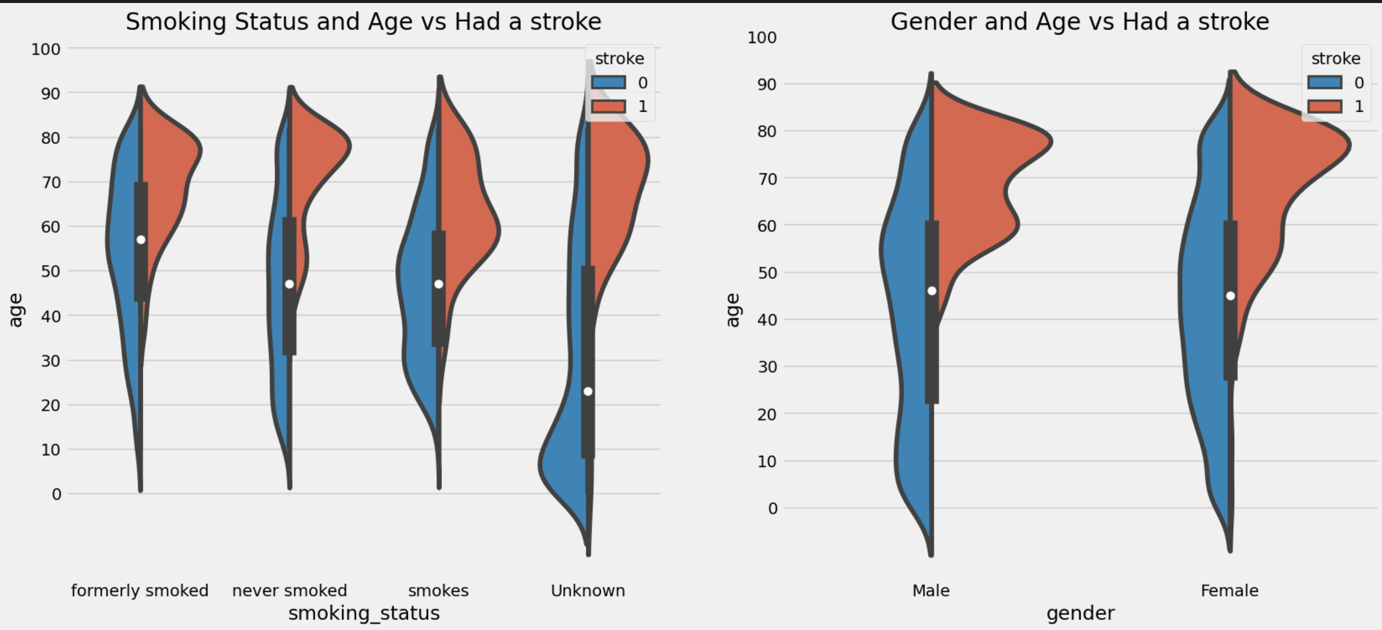
Violin plot -
Left plot Interpretation: This subplot helps visualize the distribution of ages for different smoking statuses, split by whether individuals had a stroke or not.
Right plot Interpretation: This subplot visualizes the distribution of ages for different genders, split by whether individuals had a stroke or not.
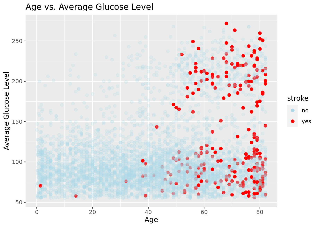
Age vs Average Glucose Level
- A combination of age and glucose levels plays a big factor into having a stroke or not. As we notice a dense population of strokes in high age plus high glucose levels.
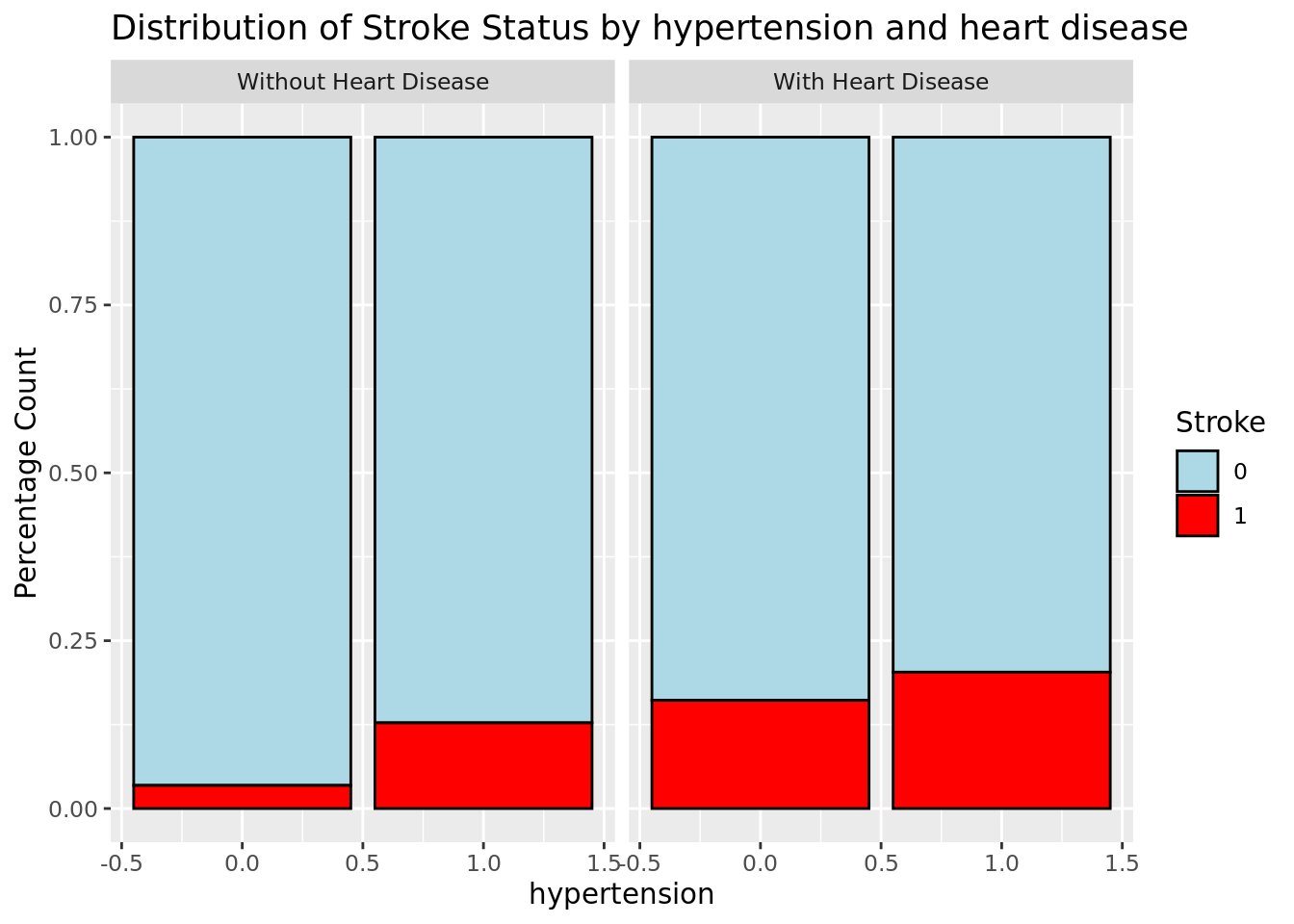
Heart disease and hypertension
- There is definitely noticeable correlation here as having more preexisting conditions will increase the chance at having a stroke, while having none conditions significantly lowers the chance.
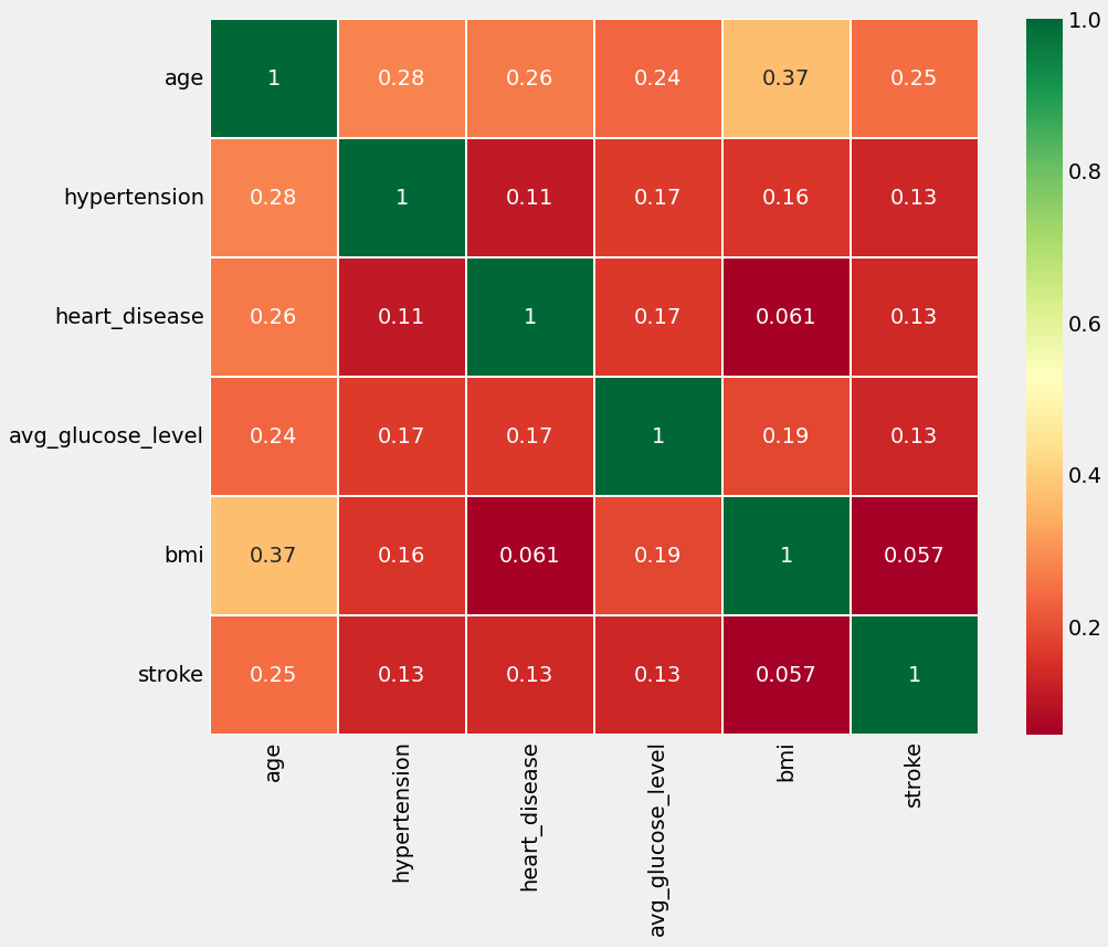
Heat map
- Heatmap colors show correlation strength: green shades mean strong, red shades mean weak. Cell numbers are correlation coefficients (0 to 1). Positive Correlation (close to 1) means variables increase together. No Correlation (close to 0) means little or no linear relationship.
Mining Method
In this project, we have used the following five classification models -
Logistic Regression
Despite its name, Logistic Regression is a binary classification algorithm. It models the probability of a binary outcome using a logistic function. In stroke prediction, logistic regression is employed to estimate the likelihood of stroke occurrence based on given features, contributing to the understanding of the relationship between various factors and stroke risk.
K-Nearest Neighbors (KNN)
KNN is a classification algorithm that classifies a data point by considering the class labels of its K-nearest neighbors in the feature space. In stroke prediction, KNN is employed to identify patterns by assessing the similarity of instances, contributing to the assessment of stroke risk based on feature patterns.
Naive Bayes
Naive Bayes is a classification algorithm based on Bayes’ theorem, assuming independence between features. In stroke prediction, it models the probability of stroke occurrence based on given features, assuming a Gaussian distribution for continuous features and feature independence.
Decision Tree
Decision trees are classification algorithms that recursively split the dataset into subsets based on significant features. They form a tree-like structure where each branch represents a decision based on specific features. In stroke prediction, decision trees are valuable for identifying key features and their interactions that contribute to predicting the likelihood of strokes.
Random Forest
Random Forests, an ensemble method, consist of multiple decision trees. They construct these trees during training and output the mode of classes or mean prediction of individual trees. In stroke prediction, Random Forests are employed to capture complex relationships within the dataset by aggregating predictions from multiple decision trees, providing a robust approach to assess stroke risk.
Code
The code splits the dataset into training and testing sets, making it ready for machine learning model training and evaluation. Features and target variables are appropriately separated for both training and testing sets.
The Logistic Regression model achieved an accuracy of approximately 95.05% on the test dataset. The accuracy score represents the proportion of correctly predicted instances out of the total instances in the test dataset. This is a high accuracy which indicates that the model performed well in predicting the target variable values on unseen data. The accuracy score is a common metric for classification models, providing a straightforward measure of predictive performance.
Code
import numpy as np
import pandas as pd
import matplotlib.pyplot as plt
import seaborn as sns
plt.style.use('fivethirtyeight')
import warnings
warnings.filterwarnings('ignore')
%matplotlib inline
from sklearn.linear_model import LogisticRegression #logistic regression
from sklearn import svm #support vector Machine
from sklearn.ensemble import RandomForestClassifier #Random Forest
from sklearn.neighbors import KNeighborsClassifier #KNN
from sklearn.naive_bayes import GaussianNB #Naive bayes
from sklearn.tree import DecisionTreeClassifier #Decision Tree
from sklearn.model_selection import train_test_split #training and testing data split
from sklearn import metrics #accuracy measure
from sklearn.metrics import confusion_matrix #for confusion matrix


# Splitting the data into training and testing
train,test=train_test_split(data,test_size=0.3,random_state=0,stratify=data['stroke'])
train_X=train[train.columns[:-1]]
train_Y=train[train.columns[-1:]]
test_X=test[test.columns[:-1]]
test_Y=test[test.columns[-1:]]
X=data[data.columns[:-1]]
Y=data["stroke"]
len(train_X), len(train_Y), len(test_X), len(test_Y)

model = LogisticRegression()
model.fit(train_X,train_Y)
prediction3=model.predict(test_X)
print('The accuracy of the Logistic Regression is',metrics.accuracy_score(prediction3,test_Y))
K Fold Cross Validation
- Implemented to check for accuracy of each models. We have selected k = 10.
Code
from sklearn.model_selection import KFold #for K-fold cross validation
from sklearn.model_selection import cross_val_score #score evaluation
from sklearn.model_selection import cross_val_predict #prediction
kfold = KFold(n_splits=10) # k=10, split the data into 10 equal parts
cv_mean=[]
accuracy=[]
std=[]
classifiers=['Logistic Regression','KNN','Decision Tree','Naive Bayes','Random Forest']
models=[LogisticRegression(),KNeighborsClassifier(n_neighbors=9),DecisionTreeClassifier(),GaussianNB(),RandomForestClassifier(n_estimators=100)]
for i in models:
    model = i
    cv_result = cross_val_score(model,X,Y, cv = kfold,scoring = "accuracy")
    cv_result=cv_result
    cv_mean.append(cv_result.mean())
    std.append(cv_result.std())
    accuracy.append(cv_result)
new_models_dataframe2=pd.DataFrame({'CV Mean':cv_mean,'Std':std},index=classifiers)
new_models_dataframe2
Results
Selected Model:
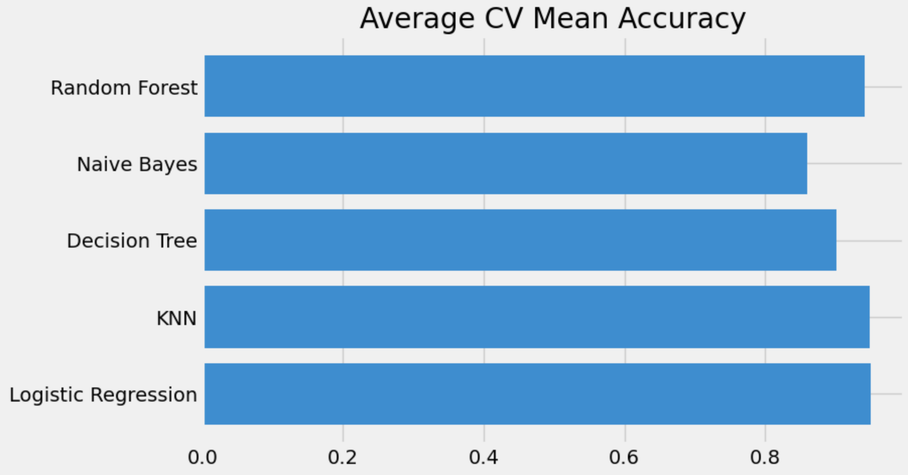
Logistic Regression has the highest accuracy of 95% from the 5 chosen models.
Hence, we have chosen logistic regression as the model to implement for the following question.
Question 2: How are certain lifestyle changes ranked on the basis of their importance in reducing the possibility of a stroke?
Approach:
The feature ranking provided by the logistic regression model with their corresponding coefficients gives insights into the impact of each feature on the likelihood of the target variable. In logistic regression, the coefficients represent the change in the log-odds of the target variable for a one-unit change in the corresponding feature.
The feature ranking provided by the logistic regression model with their corresponding coefficients gives insights into the impact of each feature on the likelihood of the target variable. In logistic regression, the coefficients represent the change in the log-odds of the target variable for a one-unit change in the corresponding feature.
Code
Code
# Get feature coefficients
feature_coefficients = model.coef_[0]

# Create a DataFrame with feature names and their corresponding coefficients
feature_coefficient_df = pd.DataFrame({'Feature': X.columns, 'Coefficient': feature_coefficients})

# Sort the DataFrame by coefficients in descending order
feature_coefficient_df = feature_coefficient_df.sort_values(by='Coefficient', ascending=False)

# Print or display the ranking order
print("Feature Ranking:")

print(feature_coefficient_df)
Results Discussion:
The feature ranking :
age_band (Coefficient: 1.187519):
For every one-unit increase in the age_band, the log-odds of the target variable increase by approximately 1.187519. Older age is associated with a higher likelihood of the target variable.
avg_glucose_level (Coefficient: 0.880860):
For every one-unit increase in avg_glucose_level, the log-odds of the target variable increase by approximately 0.880860. Higher average glucose levels are associated with a higher likelihood of the target variable.
hypertension (Coefficient: 0.551390):
Individuals with hypertension have a log-odds of the target variable approximately 0.551390 higher than those without hypertension. Hypertension is associated with a higher likelihood of the target variable.
heart_disease (Coefficient: 0.288187):
Individuals with heart disease have a log-odds of the target variable approximately 0.288187 higher than those without heart disease. Heart disease is associated with a higher likelihood of the target variable.
gender (Coefficient: 0.073007):
Being of the male gender is associated with a log-odds of the target variable approximately 0.073007 higher than being of the female gender. Gender has a positive but relatively small association with the likelihood of the target variable.
smoking_status (Coefficient: -0.053451):
For every one-unit increase in smoking_status, the log-odds of the target variable decrease by approximately 0.053451. Smoking is associated with a lower likelihood of the target variable.
bmi (Coefficient: -0.211967):
For every one-unit increase in BMI, the log-odds of the target variable decrease by approximately 0.211967. Higher BMI is associated with a lower likelihood of the target variable.