Load Libraries
suppressWarnings(library(tidyverse))
library(knitr)
library(lubridate)
library(ggplot2)
library(dplyr)
library(rpart)
library(rpart.plot)suppressWarnings(library(tidyverse))
library(knitr)
library(lubridate)
library(ggplot2)
library(dplyr)
library(rpart)
library(rpart.plot)data <- read.csv("data/study_data.csv")
# Filter the data to include only classes with one section
filtered_data1 <- data %>% filter(Sections <= 1)
# Categorize DEW_COUNT based on the mean value of Percent.DEW
filtered_data1$DEW_COUNT[filtered_data1$Percent.DEW <= 12.2] <- 'Low'
filtered_data1$DEW_COUNT[filtered_data1$Percent.DEW > 12.2] <- 'High'
# Convert DEW_COUNT to a factor variable
filtered_data1$DEW_COUNT <- as.factor(filtered_data1$DEW_COUNT)
# Select relevant columns for the decision tree
tree_data <- select(filtered_data1, DEW_COUNT, Full_Online, Hybrid, Live_Online, Reg_Session, Monday,Tuesday, Wednesday, Thursday, Friday, Saturday, Sunday, Early_Morning, Mid_Morning, Early_Afternoon, Mid_Afternoon, Evening, Asynchronous )
# Convert selected columns to logical (TRUE/FALSE) values
col_names <- c("Full_Online", "Hybrid", "Live_Online", "Reg_Session", "Monday", "Tuesday", "Wednesday", "Thursday", "Friday", "Saturday", "Sunday", "Early_Morning", "Mid_Morning", "Early_Afternoon", "Mid_Afternoon", "Evening", "Asynchronous" )
tree_data[col_names] <- sapply(tree_data[col_names], as.logical)# Check for missing values in the dataset
missing_values <- colSums(is.na(tree_data))
print(missing_values) DEW_COUNT Full_Online Hybrid Live_Online Reg_Session
0 0 0 0 0
Monday Tuesday Wednesday Thursday Friday
0 0 0 0 0
Saturday Sunday Early_Morning Mid_Morning Early_Afternoon
0 0 0 0 0
Mid_Afternoon Evening Asynchronous
0 0 0 # Display a summary of the dataset
summary(tree_data) DEW_COUNT Full_Online Hybrid Live_Online Reg_Session
High:1525 Mode :logical Mode :logical Mode :logical Mode :logical
Low :2403 FALSE:3126 FALSE:3479 FALSE:2948 FALSE:478
TRUE :802 TRUE :449 TRUE :980 TRUE :3450
Monday Tuesday Wednesday Thursday
Mode :logical Mode :logical Mode :logical Mode :logical
FALSE:2716 FALSE:2278 FALSE:2668 FALSE:2285
TRUE :1212 TRUE :1650 TRUE :1260 TRUE :1643
Friday Saturday Sunday Early_Morning
Mode :logical Mode :logical Mode :logical Mode :logical
FALSE:3314 FALSE:3928 FALSE:3928 FALSE:3333
TRUE :614 TRUE :595
Mid_Morning Early_Afternoon Mid_Afternoon Evening
Mode :logical Mode :logical Mode :logical Mode :logical
FALSE:3201 FALSE:3316 FALSE:3025 FALSE:3665
TRUE :727 TRUE :612 TRUE :903 TRUE :263
Asynchronous
Mode :logical
FALSE:3100
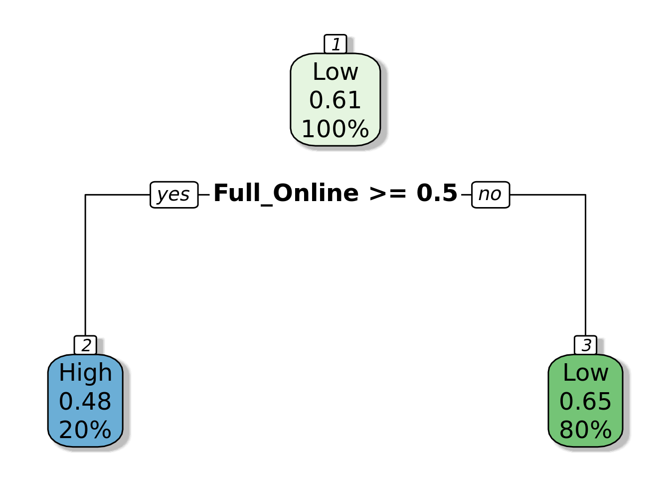
TRUE :828 # Build a decision tree
tree_default <- tree_data %>%
rpart(DEW_COUNT ~ ., data = .)
# Plot the decision tree and save it as a PNG file
png("images/decision_tree.png", width = 1000, height = 600)
rpart.plot(tree_default, box.palette = "auto", shadow.col = "gray", nn = TRUE, roundint = FALSE, cex = 1.5)
dev.off()png
2 # Plot the decision tree
rpart.plot(tree_default, box.palette = "auto", shadow.col = "gray", nn = TRUE, roundint = FALSE, cex = 1.5)